Feature selection via reinforcement learning strategies

Feature selection is a crucial step in the process of building a machine learning model. Choosing good features for the model and the task we want to accomplish can improve performance.

Feature selection is particularly important if we are dealing with a high-dimensional dataset. It enables the model to learn faster and better. The idea is to find the optimal number of features and the most meaningful features.
In this article, we will introduce and implement a new feature selection method using reinforcement learning. We will first discuss reinforcement learning, especially Markov decision processes. It is a very new method in the field of data science, especially for feature selection. Then we will introduce its implementation and how to install and use the python library (FSRLearning). Finally, we will use a simple example to demonstrate the process.
Reinforcement Learning: Markov Decision Problem for Feature Selection
Reinforcement Learning (RL) techniques can be very effective in solving problems like game solving. The concept of RL is based on Markov Decision Process (MDP). The point here is not to go into the definition but to get a general idea of how it works and how it can be useful for our problem.
The idea behind reinforcement learning is that the agent starts in an unknown environment. It takes actions to complete a task. Some actions are chosen more often based on the agent's current state and the actions it has chosen previously. The agent receives a reward for each new state it reaches and the actions it has taken. Here are the main parameters we need to define for feature selection:
Status, Action, Reward, How to Choose Action
First, a state is a subset of the features present in the dataset. For example, if the dataset has three features (age, gender, height) plus a label, the possible states are as follows:
[]                                             --> Empty set
 [Age], [Gender], [Height]                       --> 1-feature set
 [Age, Gender], [Gender, Height], [Age, Height] --> 2-feature set
[Age, Gender, Height] --> All-feature set- 1.
- 2.
- 3.
- 4.
The order of features in a state does not matter, we have to think of it as a set, not a list of features.
For actions, we can go from a subset to any subset of features that have not yet been explored. In feature selection problems, the action is to select features that have not yet been explored in the current state and add them to the next state. Here are some possible actions:
[Age] -> [Age, Gender]
[Gender, Height] -> [Age, Gender, Height]- 1.
- 2.
Here is an example of an impossible action:
[Age] -> [Age, Gender, Height]
 [Age, Gender] -> [Age]
[Gender] -> [Gender, Gender]- 1.
- 2.
- 3.
We have defined states and actions, but not rewards. A reward is a real number that evaluates the quality of a state.
In a feature selection problem, one possible reward is the improvement in the accuracy metric of the same model by adding new features. Here is an example of how the reward is calculated:
[Age] --> Accuracy = 0.65
 [Age, Gender] --> Accuracy = 0.76
Reward(Gender) = 0.76 - 0.65 = 0.11- 1.
- 2.
- 3.
For each state we visit for the first time, a classifier (model) is trained using a set of features. This value is stored in the state and the corresponding classifier. Training a classifier is a time-consuming and laborious process, so we only train it once. Because the classifier does not consider the order of the features, we can view this problem as a graph instead of a tree. In this example, the reward for the action of selecting "gender" as a new feature for the model is the difference in accuracy between the current state and the next state.

In the above diagram, each feature is mapped to a number (“age” is 1, “gender” is 2, “height” is 3). How do we choose the next state from the current state or how do we explore the environment?
We have to find the optimal approach because if we explore all possible feature sets in a problem with 10 features, then the number of states will be
10! + 2 = 3 628 802- 1.
The +2 here is because we consider an empty state and a state that contains all possible features. We can't train a model on each state, it's impossible to do, and this is only 10 features, if there are 100 features, then it's basically unsolvable.
However, in the reinforcement learning method, we do not need to train a model in all states. We need to determine some stopping conditions for this problem, such as randomly selecting the next action from the current state with a probability of epsilon (between 0 and 1, usually around 0.2), otherwise select the action that maximizes the function. For feature selection, it is the average value of the reward that each feature brings to the model accuracy.
The greedy algorithm here consists of two steps:
1. With probability epsilon, we randomly select the next state from the possible neighbors of the current state
2. Select the next state so that the features added to the current state contribute the most to the accuracy of the model. To reduce time complexity, a list containing the values of each feature can be initialized. This list is updated every time a feature is selected. Using the following formula, the update is very ideal:

AORf: The average reward brought by feature “f”
K: the number of times f is selected
V(F): The state value of the feature set F (for the sake of simplicity, this article will not go into detail)
So we want to find out which feature gives the model the highest accuracy. That's why we need to go through different states and evaluate the most globally accurate value of the model features in many different environments.
Since the goal is to minimize the number of states visited by the algorithm, the fewer unvisited states we visit, the fewer models we need to train with different feature sets. Since training a model to achieve accuracy is the most expensive method from a time and computing power perspective, we want to minimize the number of training runs.
In any case, the algorithm will stop at the final state (the set containing all features) and we want to avoid reaching this state because it is the most expensive to train a model on.
The above is our description of reinforcement learning for feature selection. Below we will introduce the implementation in Python in detail.
Python library for feature selection and reinforcement learning
There is a python library that allows us to solve this problem directly. But first we need to prepare the data
We use data directly from the UCI Machine Learning Repository:
#Get the pandas DataFrame from the csv file (15 features, 690 rows)
 australian_data = pd.read_csv('australian_data.csv', header=None)

 #DataFrame with the features
 X = australian_data.drop(14, axis=1)

 #DataFrame with the labels
y = australian_data[14]- 1.
- 2.
- 3.
- 4.
- 5.
- 6.
- 7.
- 8.
Then install the libraries we use
pip install FSRLearning- 1.
Direct import
from FSRLearning import Feature_Selector_RL- 1.
The Feature_Selector_RL class can create a feature selector. We need the following parameters
feature_number (integer): the number of features in DataFrame X
feature_structure (dictionary): dictionary for graph implementation
eps (float [0;1]): The probability of randomly selecting the next state, 0 is the greedy algorithm, 1 is the random algorithm
alpha (float [0;1]): controls the update rate, 0 means no update, 1 means frequent update
gamma (float[0,1]): The adjustment factor for the next state observation, 0 for myopic behavior state, 1 for hyperopic behavior
nb_iter (int): the number of sequences to traverse the graph
starting_state ("empty" or "random"): If "empty", the algorithm starts from an empty state, if "random", the algorithm starts from a random state in the graph
All parameters are tunable, but for most problems around 100 iterations is fine, and an epsilon value of around 0.2 is usually sufficient. The starting state is useful for exploring the graph more efficiently, but it is very dataset dependent, so both values can be tested.
We can simply initialize the selector with the following code:
fsrl_obj = Feature_Selector_RL(feature_number=14, nb_iter=100)- 1.
As with most ML libraries, the training algorithm is very simple:
results = fsrl_obj.fit_predict(X, y)- 1.
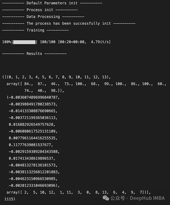
Here is an example of the output:

The output is a 5-tuple that looks like this:
Index of features in DataFrame X (similar to mapping)
The number of times the feature is observed
The average reward of all features after all iterations
Sort features from least important to most important (here 2 is the least important feature and 7 is the most important feature)
Number of states accessed globally
You can also compare to Scikit-Learn's RFE selector. It takes as input X, y, and the result of the selector.
fsrl_obj.compare_with_benchmark(X, y, results)- 1.
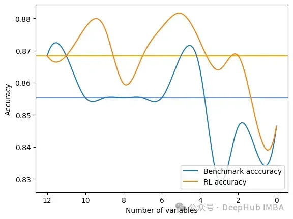
The output is the result after each step of the selection of the global metric for RFE and FSRLearning. It also outputs a visual comparison of the model accuracy, where the x-axis represents the number of selected features and the y-axis represents the accuracy. The two horizontal lines are the median accuracy of each method.

Average benchmark accuracy : 0.854251012145749, rl accuracy : 0.8674089068825909
 Median benchmark accuracy : 0.8552631578947368, rl accuracy : 0.868421052631579
 Probability to get a set of variable with a better metric than RFE : 1.0
Area between the two curves : 0.17105263157894512- 1.
- 2.
- 3.
- 4.
It can be seen that the RL method always provides a better feature set for the model than RFE.
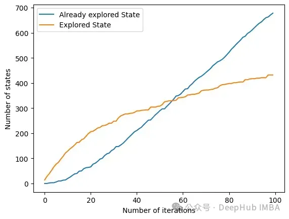
Another interesting method is get_plot_ratio_exploration. It draws a graph comparing the number of nodes visited and the number of nodes visited in an exact sequence of iterations.

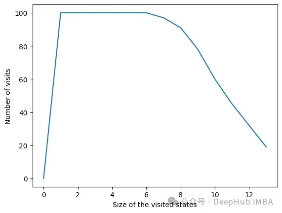
Due to the setting of stopping conditions, the time complexity of the algorithm decreases exponentially. Even if the number of features is large, convergence will be found quickly. The following figure shows the number of times a set of a certain size is visited.

In all iterations, the algorithm visits states containing 6 variables or less. Beyond 6 variables, we can see that the number of states reached is decreasing. This is a good behavior because training a model with a small feature set is faster than training a model with a large feature set.
Summarize
We can see that the RL method is very effective for maximizing the metric of the model. It always converges to an interesting subset of features very quickly. This method is very easy and fast to implement in ML projects using the FSRLearning library.