Have you learned the change point detection algorithm for time series?

Suppose you are exercising and using a digital device to monitor your heart rate. You run a quarter mile, then walk for ten minutes, and then run another quarter mile. Your heart rate may look like the time series in Figure (1). The figure shows a period of high heart rate, a period of low heart rate, and then a return to a high heart rate. The sudden change in the time series tells us that your activity state has changed significantly.
 figure 1)
Change point detection refers to the points where a significant structural break or shift has occurred in the time series. These changes may be caused by external factors such as data generation, technology, or consumer behavior. Detecting these change points is very important because it helps us understand and quantify the changes. We need to detect these changes in a timely and accurate manner and issue alerts immediately.
Change point detection (CPD) is called change point detection. Its basic definition is that in a sequence or process, when a statistical characteristic (distribution type, distribution parameter) changes at a certain point in time due to systematic factors rather than accidental factors, we call this time point a change point. Change point identification is to estimate the position of the change point using statistics, statistical methods, or machine learning methods.
CPD has a wide range of applications in many fields, including finance, healthcare, and environmental monitoring. Among them, it can help identify changes in product or service quality during quality control, and can also be applied to medical diagnosis to help determine changes in a patient's health or disease. For example, patients in the intensive care unit (ICU) need to have their heart rate monitored continuously, and timely detection of any changes in heart rate and prompt response from doctors is crucial to the patient's life.
In CPD, we mainly look for points in the time series where basic statistical properties (such as mean, variance or autocorrelation) change significantly. Although there are many algorithms to detect these change points, an important aspect is to clarify the data type (i.e. real-time data stream or offline data) because this will determine the choice and development of the algorithm.
Whether the algorithm depends on real-time or offline data
The way the CPD algorithm works depends on the type of data, i.e. real-time data or offline data. For offline data, we can use historical data to analyze the entire sequence, in which case offline CPD is applicable. Offline CPD involves analyzing an already collected data set and is suitable for historical data analysis or detecting anomalies in a data set.
However, in a real-time environment, we need to detect change points quickly, when no historical data is available. For example, a drone sends a stream of location information to home devices every second, and we cannot wait and collect data for a long time to detect changes. Online video streaming is another example. Real-time CPD requires monitoring the data stream as it arrives and responding immediately. This situation often occurs in many real-time applications, such as financial market monitoring, fraud detection, or critical infrastructure monitoring.
For offline CPD, we will introduce the Ruptures Python module. For live CPD, we will demonstrate the changefinder module.
Generate data
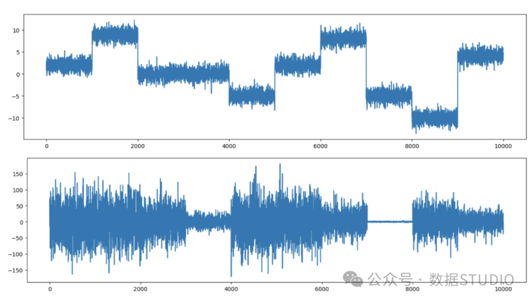
Generate two time series to test the algorithm.
- Constant variance (ts1): There are ten data segments with constant variance.
- Varying variance (ts2): There are ten data segments, but the variance varies.
import numpy as np
import pandas as pd
import random
import matplotlib.pyplot as plt

# Example 1: 恒定方差
ts1 = []
mu, sigma, seg = 0.0, 1.0, 1000
for i in range(10):
    ts = np.random.normal(mu, sigma, seg) + np.random.randint(low=-10, high=10)
    ts1 = np.append(ts1,ts, axis=0)

plt.figure(figsize=(16,4))
plt.plot(ts1)


# Example 2: 变化方差
ts2 = []
mu, sigma, seg = 0.0, 1.0, 1000
for i in range(10):
    sig = np.random.randint(low=1, high=50)
    ts = np.random.normal(mu, sigma * sig, seg)
    ts2 = np.append(ts2,ts, axis=0)

plt.figure(figsize=(16,4))
plt.plot(ts2)- 1.
- 2.
- 3.
- 4.
- 5.
- 6.
- 7.
- 8.
- 9.
- 10.
- 11.
- 12.
- 13.
- 14.
- 15.
- 16.
- 17.
- 18.
- 19.
- 20.
- 21.
- 22.
- 23.
- 24.
- 25.
- 26.
Figure (2) shows the time series. The change points in the first time series are easier to find, while the change points in the second time series are more difficult to find.
 Figure (2): Constant variance time series and varying variance time series
Offline-ruptures module
In offline analysis, we can use the historical data of the time series. For CPD, we can apply the concept of linear regression. However, if there are change points, the straight line cannot fit the data well, and the segmented line can better fit the data. An intuitive algorithm to build the segmented line is to determine the change points as breakpoints. This method is called Exact Linear Time (PELT) .
Figures (3.A) and (3.B) explain PELT. There is a change point and two segments in the time series (shown in blue). The orange line represents the regression line, while the orange vertical line represents the distance of each point (represented by white circles) to the regression line. The regression line is determined by minimizing the sum of the distances of all data points.
 Figure (3): Pruned Exact Linear Time (PELT)
In Figure (3.B), the segmented line fits the data better. The sum of the distances from the actual points to the line is smaller than the sum of the distances in Figure (3.A). The algorithm finds the appropriate change point by sliding from the left side of the time series to the right side so that the sum of the distances or errors is minimized.
Below is the algorithm used to search for the number and location of change points. C(.) represents the distance or cost function. We also need to control not to create too many segments to prevent overfitting the time series. Therefore, the b(β) term acts as a parameter that penalizes the number of segments to prevent the search from generating too many segments.
 picture
The algorithm is coded in the Python module ruptures.
For the first use, you need to install it with pip install ruptures.
(1) Constant variance
# !pip install ruptures
import ruptures as rpt

# Detect the change points
algo1 = rpt.Pelt(model="rbf").fit(ts1)
change_location1 = algo1.predict(pen=10)

# Point the change points:
def plot_change_points(ts,ts_change_loc):
    plt.figure(figsize=(16,4))
    plt.plot(ts)
    for x in ts_change_loc:
        plt.axvline(x,lw=2, color='red')

plot_change_points(ts1,change_location1)- 1.
- 2.
- 3.
- 4.
- 5.
- 6.
- 7.
- 8.
- 9.
- 10.
- 11.
- 12.
- 13.
- 14.
- 15.
Figure (4) shows that the algorithm detected all ten change points.
 Figure (4): All ten change points of the constant variance time series are detected
Is CPD still valid when the variance changes over time?
(2) Variance of change
Figure (5) shows that the PELT algorithm found the change points at [3000, 4000, 6005, 7000, 8000, 8995, 10000].
# detect the change points #
algo2 = rpt.Pelt(model="rbf").fit(ts2)
change_location2 = algo2.predict(pen=10)
change_location2

# Plot the change points #
plot_change_points(ts2,change_location2)- 1.
- 2.
- 3.
- 4.
- 5.
- 6.
- 7.
We know there should be two change points [1000, 2000, 5000]. However, since the data before and after these points are too similar, PELT cannot detect these differences.
 Figure (5): PELT detects some change points in the time series of changing variance
When using the PELT algorithm, finding the change points in Figure (4) and Figure (5) may require relatively long processing time, especially for Figure (5). This may not meet the needs of real-time streaming data. Therefore, for real-time applications, we designed a Python module called changefinder.
Real-time CPD
Time series can be described by an autoregressive (AR) moving average process. In the AR model, the next data point is a weighted moving average of past data points with random noise. Specifically, the following formula represents the AR model, where θi is the weight of the past p data points.
 picture
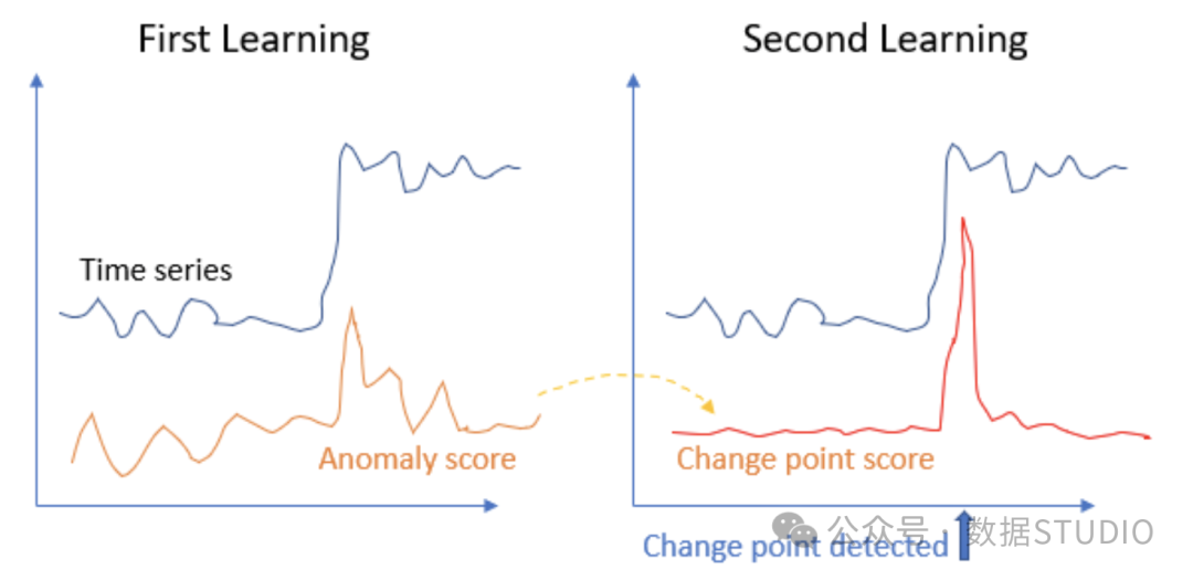
If there is a change point, then the autoregressive process before and after the change point is expected to be different. Based on this intuition, Yamanishi & Takeuchi proposed the Sequential Discounted Autoregressive (SDAR) learning algorithm, which drove their research. The SDAR method consists of two learning stages. In the first learning stage, it generates an intermediate score called "anomaly score". In the second learning stage, it generates a "change point score" that can detect change points. The following is an overview of the algorithm.
- AR Model 1 takes in a chunk of data t = 1, ..., N and builds an AR (auto-regression) model. It then generates an "anomaly score" which is the difference between the AR predicted Xt value and the actual data Xt. Note that only N data points are extracted in this step. Since it does not use the entire historical data, it is set up for online data streams.
- The first smoothing process will be very unstable and produce false signals. The algorithm generates a moving average Yt for the anomaly score to smooth out the outliers.
- The second AR model builds an AR model for Yt and generates another "anomaly score" based on the newly built AR model and Yt.
- In the second smoothing, the new anomaly score will also fluctuate. The algorithm will generate a moving average to smooth it. As shown in Figure (6), the final score generated is called the "change point score".
This algorithm does not require the entire time series to detect change points, thus significantly reducing the computation time.
 Figure (6): Sequential Discounted Auto-Regression (SDAR) learning algorithm
Let’s study two time series situations.
(1) Constant variance
The preceding code works for a constant variance time series (ts1). Changefinder requires three parameters:
- r: discount rate (0 to 1). A higher discount rate will cause past time series to decrease rapidly, meaning you may not want to learn from past time series. It is recommended to set it to 0.01. Since the discount rate is not very sensitive, setting it to 0.01 or 0.05 is OK, you can try it yourself.
- order: AR model order
- smooth: The size of the most recent N data used to calculate the smoothed moving average.
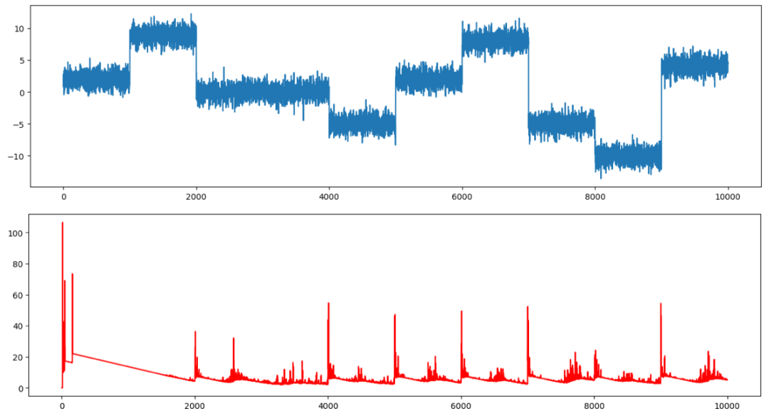
In the changefinder module, we are interested in the change point score, which shows whether the time series deviates abruptly from its normality.
# !pip install changefinder
import changefinder

def findChangePoints(ts, r, order, smooth):
    '''
       r: Discounting rate
       order: AR model order
       smooth: smoothing window size T
    '''
    cf = changefinder.ChangeFinder(r=r, order=order, smooth=smooth)
    ts_score = [cf.update(p) for p in ts]
    plt.figure(figsize=(16,4))
    plt.plot(ts)
    plt.figure(figsize=(16,4))
    plt.plot(ts_score, color='red')
    return(ts_score)

ts_score1 = findChangePoints(ts1, r = 0.01, order = 3, smooth = 5)- 1.
- 2.
- 3.
- 4.
- 5.
- 6.
- 7.
- 8.
- 9.
- 10.
- 11.
- 12.
- 13.
- 14.
- 15.
- 16.
- 17.
- 18.
Figure (7) shows ts1 in the first figure, and the red time series in the second figure is the change point score. The locations where changes occur are those with large change point scores.
 Figure (7): Change point scores of the SDAR algorithm for constant variance time series
Here I have printed out the top 20 positions (you can select more).
ts_change_loc1 = pd.Series(ts_score1).nlargest(20)
ts_change_loc1 = ts_change_loc1.index
np.sort(ts_change_loc1)- 1.
- 2.
- 3.
array([ 11, 12, 13, 42, 43, 159, 160, 4001, 4008,
      5001, 5007, 5008, 6007, 6008, 7000, 7001,
9000, 9001, 9007, 9008])- 1.
- 2.
- 3.
Overall, the algorithm does a pretty good job considering this is a real-time operation. It detects many change points, but misses the 1000, 2000, and 8000 points. This is because the frequencies of the data before and after these points are too similar to qualify as different. When you run the code, you may find that the computation time is much less than the PELT method of the Fracture module.
The time series with change points are plotted in Figure (8).
def plot_change_points(ts,ts_change_loc):
    plt.figure(figsize=(16,4))
    plt.plot(ts)
    for x in ts_change_loc:
        plt.axvline(x,lw=2, color='red')

plot_change_points(ts1,ts_change_loc1)- 1.
- 2.
- 3.
- 4.
- 5.
- 6.
- 7.
 Figure (8): The SDAR algorithm detected most of the 10 change points in the constant variance time series.
(2) Variance of change
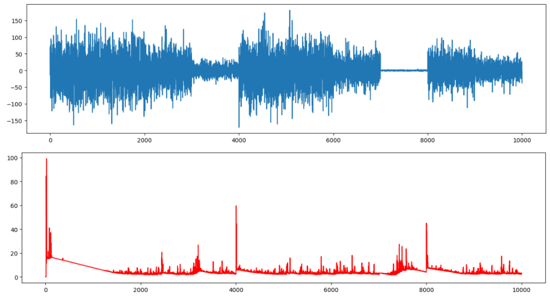
The change points in the time series of changing variance are hard to find. As shown in Figure (9), ts2 looks like three or four clusters instead of the ten clusters we designed.
ts_score2 = findChangePoints(ts2, r = 0.01, order = 3, smooth = 5)- 1.
Figure (9) shows the ts2 in the first figure and the change point scores in the second figure. There are three high points.
 Figure (9): SDAR algorithm change point score for a time series with varying variance
Print out the top 20 positions.
ts_change_loc2 = pd.Series(ts_score2).nlargest(20)
ts_change_loc2 = ts_change_loc2.index
np.sort(ts_change_loc2)- 1.
- 2.
- 3.
array([ 11, 12, 13, 19, 20, 21, 22, 80, 81, 107,
        108, 117, 4003, 4004, 4010, 4011, 8000,
8001, 8007, 8008])*- 1.
- 2.
- 3.
This method identified the change points at 1, 4000, and 8000, but missed the change points at 1000, 2000, 3000, 5000, 6000, 7000, and 9000.
plot_change_points(ts2,ts_change_loc2)- 1.
If we observe Figure (10) visually, we can see that there are three or four clusters. The SDAR algorithm can detect these major change points.
 Figure (10): SDAR algorithm detects the main change points of the time series of changing variance