Warning! Long-distance LiDAR sensing
2024.02.02

This article is reprinted with permission from the Autonomous Driving Heart public account. Please contact the source for reprinting.
I. Introduction
After I opened Tucson AI Day last year, I have always wanted to summarize the work I have done on long-distance perception in the past few years in text form. I just have time recently, so I wanted to write an article to record the research process in the past few years. The contents mentioned in this article are all in the Tucson AI Day video [0] and published papers, and do not involve specific engineering details and other technical secrets.
As we all know, Tucson is engaged in self-driving trucks, and the braking distance and lane change time of trucks are much longer than that of cars. So if Tucson has any unique technology that is different from other self-driving companies, long-distance sensing must be one of them. I am responsible for LiDAR sensing in Tucson, and I will specifically talk about using LiDAR for long-distance sensing.
When I first joined the company, the mainstream LiDAR sensing solution was generally the BEV solution. However, this BEV is not the BEV that everyone is familiar with. I personally think Tesla’s BEV perception should be called “multi-view camera fusion technology in the BEV space”, and the LiDAR BEV here refers to projecting the LiDAR point cloud onto the BEV. space, and then connect 2D convolution + 2D detection head for target detection. The earliest record of the BEV solution that I can find is the paper MV3D[1] published by Baidu at CVPR17. Most of the subsequent work, including the solutions actually used by most companies that I know, will eventually be projected into the BEV space. Testing can generally be included in the BEV program.
 BEV perspective features used by MV3D[1]
One of the great benefits of the BEV solution is that it can directly apply mature 2D detectors, but it also has a fatal shortcoming: it limits the sensing range. As you can see from the picture above, because a 2D detector is to be used, it must form a 2D feature map. At this time, a distance threshold must be set for it. In fact, there are still LiDAR points outside the range of the picture above, but was discarded by this truncation operation. Is it possible to increase the distance threshold until the location is covered? It’s not impossible to do this, but LiDAR has very few point clouds in the distance due to problems such as scanning mode, reflection intensity (attenuating with distance to the fourth power), occlusion, etc., so it is not cost-effective.
This problem of the BEV solution has not attracted attention in the academic community. This is mainly a problem of the data set. The annotation range of mainstream data sets is usually less than 80m (nuScenes 50m, KITTI 70m, Waymo 80m). At this distance, the BEV feature map It doesn't need to be big. However, the mid-range LiDAR used in the industry can generally achieve a scanning range of 200m, and in recent years, several long-range LiDARs have been released, which can achieve a scanning range of 500m. It is noted that the area and calculation amount of the feature map increase quadratically with distance. Under the BEV scheme, the calculation amount of 200m is almost unbearable, let alone 500m.
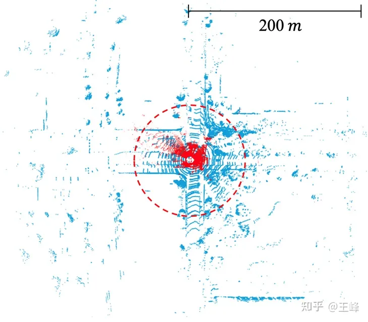
Scanning range of lidar in public datasets. KITTI (red dot, 70m) vs. Argoverse 2 (blue dot, 200m)
After recognizing the limitations of the BEV solution, we conducted years of research before finally finding a viable alternative. The research process has not been smooth sailing, and I have experienced many setbacks. Papers and reports generally only talk about success and not failure. However, the experience of failure is also precious, so blogging has become a better medium. Click below Let’s talk about the timeline in turn.
2. Point-based solution
At CVPR19, Hong Kong Chinese published an article about the Point-based detector PointRCNN [2]. It is calculated directly on the point cloud. It calculates where the point cloud is scanned. There is no process of taking BEV, so this type of point -based solution can theoretically achieve long-distance sensing.
But we found a problem after trying it. The number of point clouds in one frame of KITTI can be downsampled to 16,000 points for detection without much loss of points. However, our LiDAR combination has more than 100,000 points in one frame. If we downsample 10 Obviously, the detection accuracy will be greatly affected. If downsampling is not performed, there are even O(n^2) operations in the backbone of PointRCNN. As a result, although it does not take bev, the calculation amount is still unbearable. These time-consuming operations are mainly due to the disordered nature of the point cloud itself, which means that all points must be traversed whether downsampling or neighborhood retrieval. Since there are many ops involved and they are all standard ops that have not been optimized, there is no hope of optimizing to real-time in the short term, so this route was abandoned.
However, this period of research was not wasted. Although the calculation amount of backbone is too large, its second stage is only performed on the foreground, so the calculation amount is still relatively small. After directly applying the second stage of PointRCNN to the first stage detector of the BEV scheme, the accuracy of the detection frame will be greatly improved. During the application process, we also discovered a small problem with it. After solving it, we summarized it and published it in an article [3] published on CVPR21. You can also check it out on this blog:
Wang Feng: LiDAR R-CNN: a fast and versatile two-stage 3D detector
3. Range-View solution
After the Point-based solution failed, we turned our attention to Range View. LiDAR back then were all mechanically rotating. For example, a 64-line lidar would scan 64 rows of point clouds with different pitch angles. For example, each row If 2048 points are scanned, a 64*2048 range image can be formed.
 Comparison of RV, BEV, and PV
Under Range View, point clouds are no longer sparse but densely arranged. Long-distance targets are only smaller on the range image, but will not be discarded, so they can theoretically be detected.
Perhaps because it is more similar to the image, the research on RV is actually earlier than BEV. The earliest record I can find is also from Baidu’s paper [4]. Baidu is really the Whampoa Military Academy of autonomous driving, whether it is RV or BEV. The earliest applications came from Baidu.
So I tried it casually at that time. Compared with the BEV method, the AP of RV dropped by 30-40 points... I found that the detection on the 2D range image was actually OK, but the output 3D frame The effect is very poor. At that time, when we analyzed the characteristics of RV, we felt that it had all the disadvantages of images: non-uniform object scales, mixed foreground and background features, and unclear long-distance target features. However, it did not have the advantage of rich semantic features in images, so I was relatively pessimistic about this solution at the time.
Because regular employees still have to do the implementation work after all, it is better to leave such exploratory issues to interns. Later, two interns were recruited to study this problem together. They tried it on the public data set, and sure enough, they also lost 30 points... Fortunately, the two interns were more capable. Through a series of efforts and reference to other After correcting some details of the paper, the points were brought to a level similar to the mainstream BEV method, and the final paper was published on ICCV21 [5].
Although the number of points has increased, the problem has not been completely solved. At that time, it has become a consensus that lidar requires multi-frame fusion to improve the signal-to-noise ratio. Because the number of points is small, long-distance targets require superimposed frames to increase the amount of information. In the BEV solution, multi-frame fusion is very simple. Just add a timestamp to the input point cloud and then superimpose multiple frames. The entire network can increase the points without changing it. However, under RV, many tricks have been changed and nothing has been achieved. Similar effect.
And at this time, LiDAR has also moved from mechanical rotation to solid/semi-solid state in terms of hardware technical solutions. Most solid/semi-solid LiDAR can no longer form a range image. Forcibly constructing a range image will lose information, so This path was eventually abandoned.
4. Sparse Voxel solution
As mentioned before, the problem with the Point-based scheme is that the irregular arrangement of point clouds makes downsampling and neighborhood retrieval problems require traversing all point clouds, resulting in excessive calculations. However, under the BEV scheme, the data is regularized but there are too many blank areas. This results in excessive computational effort. Combining the two, performing voxelization in dotted areas to make it regular, and not expressing in undotted areas to prevent invalid calculations seems to be a feasible path. This is the sparse voxel solution.
Because Yan Yan, the author of SECOND[6], joined Tucson, we tried the backbone of sparse conv in the early days. However, because spconv is not a standard op, the spconv implemented by ourselves is still too slow to be implemented in real time. Detection is sometimes even slower than dense conv, so it is put aside for the time being.
Later, the first LiDAR capable of scanning 500m: Livox Tele15 arrived, and the long-range LiDAR sensing algorithm was imminent. I tried the BEV solution but it was too expensive, so I tried the spconv solution again because Tele15’s fov It is relatively narrow, and the point cloud in the distance is also very sparse, so spconv can barely achieve real-time performance.
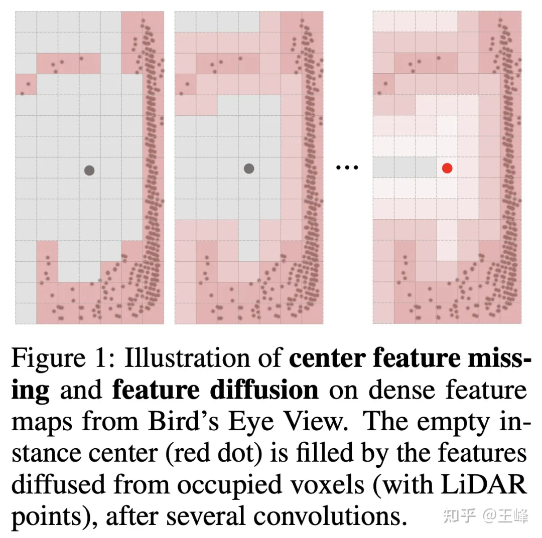
But if you don’t shoot bev, the detection head cannot use the more mature anchor or center assign in 2D detection. This is mainly because the lidar scans the surface of the object, and the center position is not necessarily a point (as shown in the figure below). Without a point, it is naturally impossible to assign a foreground target. In fact, we have tried many assign methods internally. We will not go into details about the actual methods used by the company here. The intern also tried an assign scheme and published it on NIPS2022 [7]. You can read his interpretation. :
The bright moon does not know the pain of separation: a fully sparse 3D object detector
But if you want to apply this algorithm to a LiDAR combination of 500m forward, 150m backward and left and right, it is still insufficient. It just so happened that the intern used to draw on the ideas of Swin Transformer and wrote an article on Sparse Transformer before chasing popularity [8]. It also took a lot of effort to brush up from more than 20 points bit by bit (thanks to the intern for guiding me, tql ). At that time, I felt that the Transformer method was still very suitable for irregular point cloud data, so I also tried it on the company's data set.
It is a pity that this method has always failed to beat the BEV method on the company's data set, and the difference is close to 5 points. Looking back now, there may be some tricks or training techniques that I have not mastered. It stands to reason that Transformer's expression ability is not weak. Yu conv, but later did not continue to try. However, at this time, the assign method has been optimized and reduced a lot of calculations, so I wanted to try spconv again. The surprising result is that directly replacing the Transformer with spconv can achieve the same accuracy as the BEV method at close range. Quite, it can also detect long-distance targets.
It was also at this time that Yan Yan made the second version of spconv[9]. The speed was greatly improved, so computing delay was no longer a bottleneck. Finally, long-distance LiDAR perception cleared all obstacles and was able to operate on the car. It started running in real time.
Later, we updated the LiDAR arrangement and increased the scanning range to 500m forward, 300m backward, and 150m left and right. This algorithm also runs well. I believe that as computing power continues to increase in the future, the calculation delay will become increasingly large. The less of a problem.
The final long-distance detection effect is shown below. You can also look at the position around 01:08:30 in the Tucson AI Day video to see the dynamic detection effect:
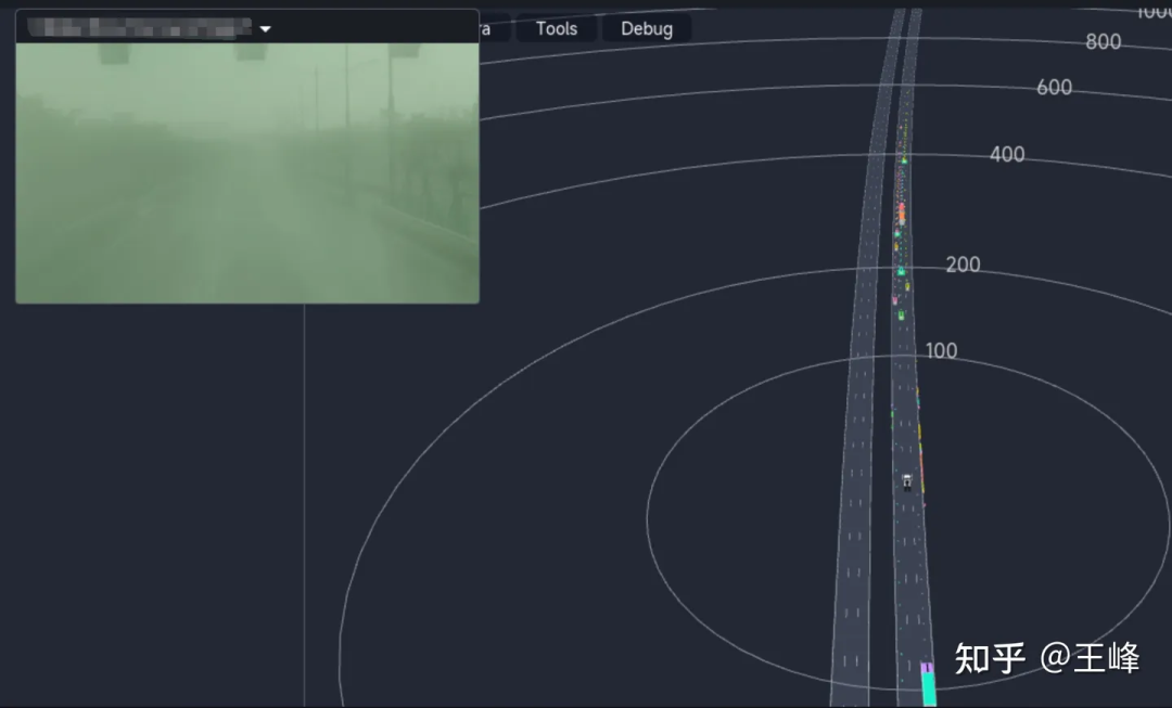
Although it is the final fusion result, because the visibility of the foggy image on this day is very low, the results basically come from LiDAR perception.
5. Postscript
From the point-based method, to the range image method, to the Transformer and sparse conv methods based on sparse voxel, the exploration of long-distance perception cannot be said to be smooth sailing, it is simply a road full of thorns. In the end, it was actually with the continuous improvement of computing power and the continuous efforts of many colleagues that we achieved this step. I would like to thank Wang Naiyan, chief scientist of Tucson, and all colleagues and interns in Tucson. Most of the ideas and engineering implementations here were not done by me. I am very ashamed. They serve more as a link between the past and the future.
It’s been a long time since I’ve written such a long article. It was written like a running account without forming a touching story. In recent years, fewer and fewer colleagues insist on doing L4, and L2 colleagues have gradually turned to purely visual research. LiDAR perception is gradually marginalized visibly to the naked eye, although I still firmly believe that one more direct ranging sensor is better. choice, but industry insiders seem to increasingly disagree. As I see more and more BEV and Occupancy on the resumes of the fresh blood, I wonder how long LiDAR sensing can continue, and how long I can persist. Writing such an article may also serve as a commemoration.
I'm crying late at night, I don't understand what I'm talking about, I'm sorry.